Concepts

Concepts#

These concepts span multiple functions in the pipeline. Understanding them helps you set up sweeps correctly and interpret results without surprises.

Aerodynamics#

AVL reports all forces and moments as dimensionless coefficients normalized by the dynamic pressure and the reference geometry declared in the .avl file header.

Nomenclature#

Symbol	Name	Typical unit
$\alpha$	Angle of attack, nose-up rotation from relative wind	deg
$\beta$	Sideslip angle, nose-right rotation from relative wind	deg
$V$	Relative wind speed	m/s or ft/s
$\rho$	Air density	kg/m³ or slug/ft³
$q = \tfrac{1}{2}\rho V^2$	Dynamic pressure	Pa or lb/ft²
$S_\text{ref}$	Reference wing area (declared in `.avl` header as `Sref`)	m² or ft²
$b$	Reference span (declared in `.avl` header as `Bref`)	m or ft
$\bar{c}$	Mean aerodynamic chord (declared in `.avl` header as `Cref`)	m or ft
$C_{(\cdot)}$	Dimensionless aerodynamic coefficient	—

$S_\text{ref}$, $b$, and $\bar{c}$ are set once in the .avl file and used by AVL as the denominators in every coefficient definition; they are reference constants, not computed quantities.

Reference Frames#

Three right-handed frames are used in aero analysis (body, stability, and wind), each a rotation of the previous.

Body axes ($x_b$, $y_b$, $z_b$): fixed to the airframe, independent of the flow, with $x_b$ out the nose, $y_b$ out the right (starboard) wing, and $z_b$ down through the belly.

Stability axes ($x_s$, $y_s$, $z_s$): body axes tilted up by $\alpha$ about the $y_b$ axis, so that $x_s$ points into the relative wind when sideslip is zero. AVL reports all forces and moments in this frame:

\[\begin{split}\begin{pmatrix}x_s\\y_s\\z_s\end{pmatrix} = \begin{pmatrix}\cos\alpha & 0 & \sin\alpha\\0 & 1 & 0\\-\sin\alpha & 0 & \cos\alpha\end{pmatrix} \begin{pmatrix}x_b\\y_b\\z_b\end{pmatrix}\end{split}\]

Wind axes ($x_w$, $y_w$, $z_w$): stability axes rotated by sideslip $\beta$ about the $z_s$ axis, so that $x_w$ is fully aligned with the relative wind in both the pitch and yaw planes:

\[\begin{split}\begin{pmatrix}x_w\\y_w\\z_w\end{pmatrix} = \begin{pmatrix}\cos\beta & -\sin\beta & 0\\\sin\beta & \cos\beta & 0\\0 & 0 & 1\end{pmatrix} \begin{pmatrix}x_s\\y_s\\z_s\end{pmatrix}\end{split}\]

Frame	Aligned with	Used for
Body ($x_b$, $y_b$, $z_b$)	Airframe geometry	Equations of motion, inertia
Stability ($x_s$, $y_s$, $z_s$)	Freestream in pitch only ($\beta = 0$ assumed)	AVL output: all coefficients here
Wind ($x_w$, $y_w$, $z_w$)	Full relative wind (both $\alpha$ and $\beta$)	True drag / lift / sideforce

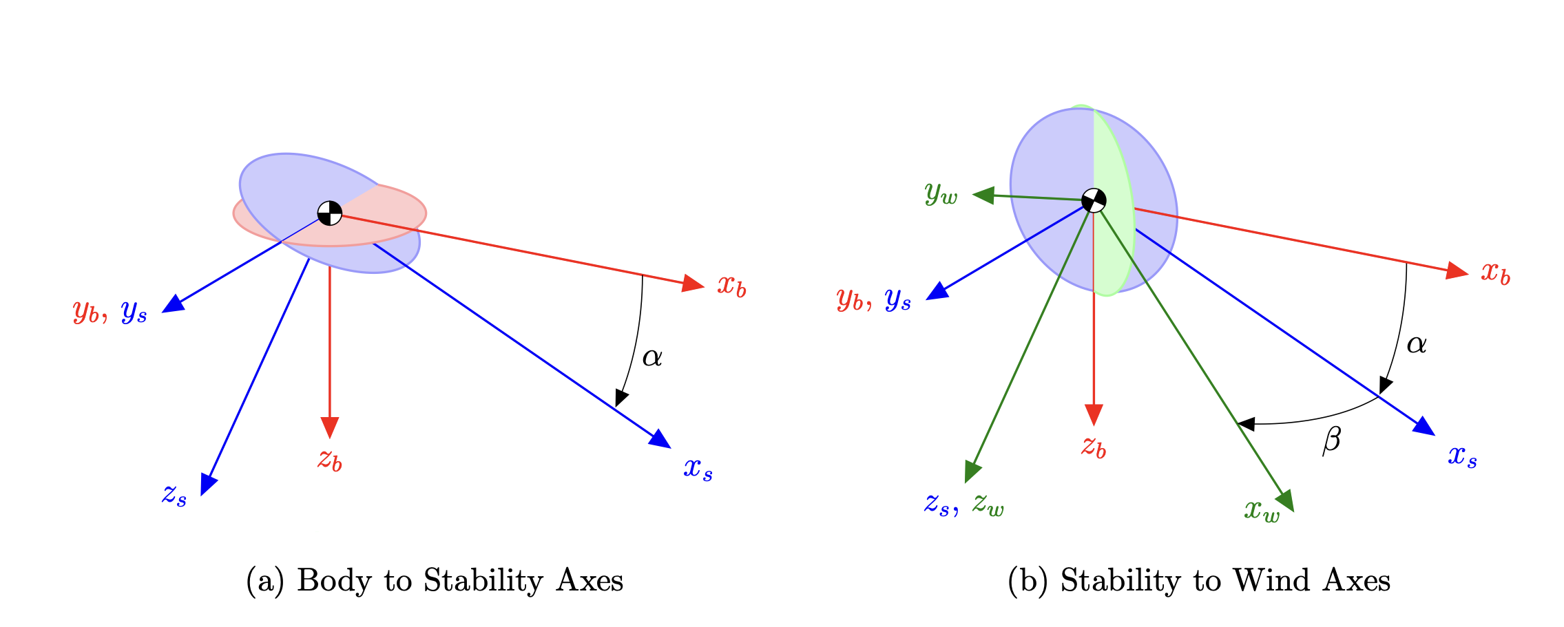
Figure 2.1: Air Vehicle Reference Frames (Borra, 2012)#

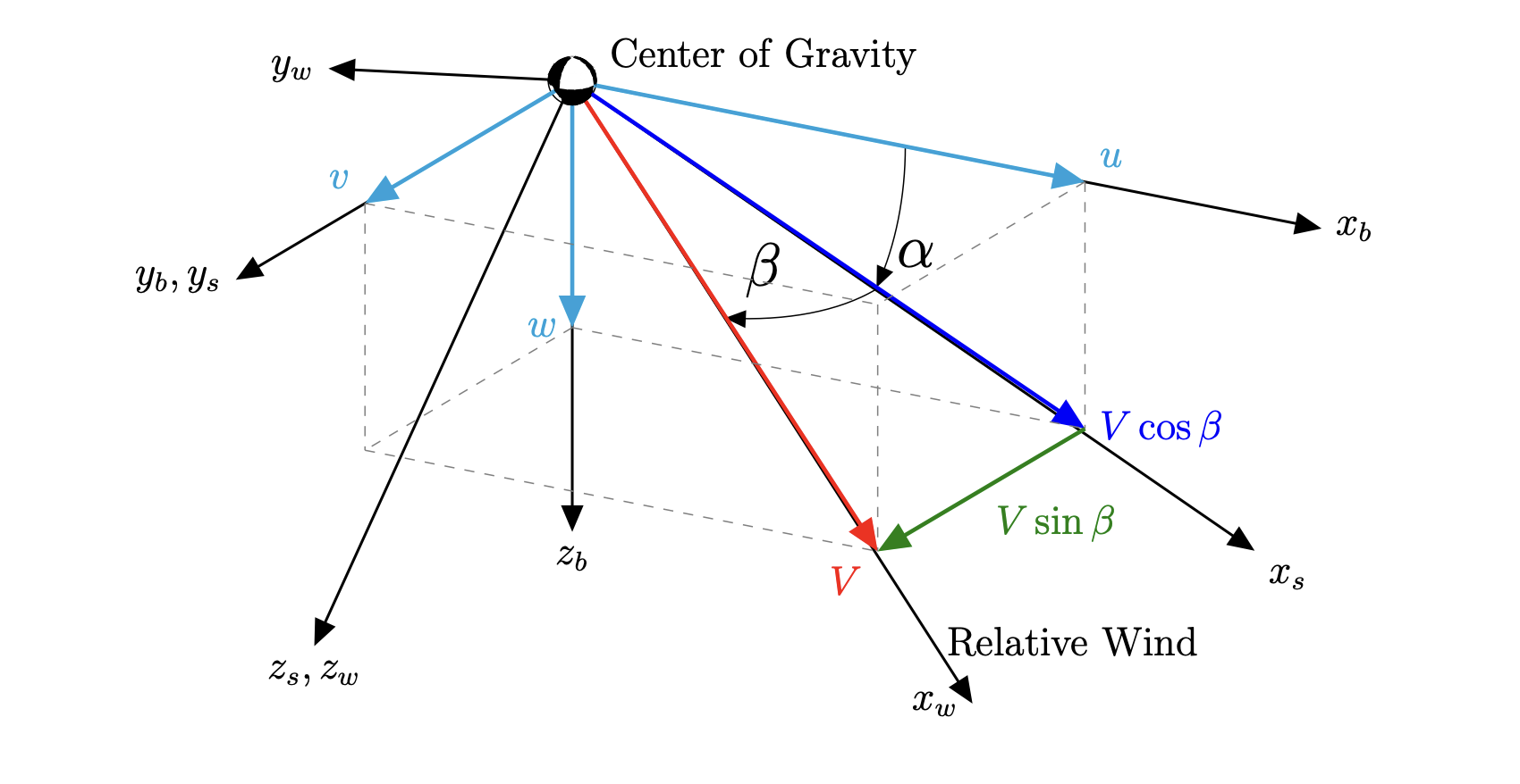
Figure 2.2: Axis Relationships: Body, Stability, and Wind Axes (Borra, 2012)#

Definitions#

Upper-case ($C_L$, $C_Y$, $C_D$) denotes forces; lower-case ($C_l$, $C_m$, $C_n$) denotes moments — standard notation in aerospace textbooks and throughout AVL output. In AVL’s .st files and AeroDatabase keys, the same symbols appear as CLtot, CDtot, Cltot, etc.; see Data Categories for the full key listing.

(1)#\[\begin{split}\begin{aligned} C_L &= F_z \;/\; (q \cdot S_\text{ref}) \\ C_Y &= F_y \;/\; (q \cdot S_\text{ref}) \\ C_D &= F_x \;/\; (q \cdot S_\text{ref}) \\ C_l &= M_x \;/\; (q \cdot S_\text{ref} \cdot b) \\ C_m &= M_y \;/\; (q \cdot S_\text{ref} \cdot \bar{c}) \\ C_n &= M_z \;/\; (q \cdot S_\text{ref} \cdot b) \end{aligned}\end{split}\]

Symbol	Name	Sense	Frame
$C_L$	Lift coefficient	positive up (opposing gravity)	stability $\equiv$ wind
$C_Y$	Side-force coefficient	positive right-wing	stability[1]
$C_D$	Drag coefficient	positive opposing relative wind	stability[1]
$C_l$	Roll-moment coefficient	positive right-wing-down	stability[1]
$C_m$	Pitch-moment coefficient	positive nose-up	stability[1]
$C_n$	Yaw-moment coefficient	positive nose-right	stability $\equiv$ wind

Normalizing Forces & Moments#

AVL normalizes forces and moments by dynamic pressure $q$ and reference geometry. The dimensional equivalents are:

(2)#\[\begin{split}\begin{aligned} L &= C_L \cdot \tfrac{1}{2}\rho V^2 \cdot S_\text{ref} \\ Y &= C_Y \cdot \tfrac{1}{2}\rho V^2 \cdot S_\text{ref} \\ D &= C_D \cdot \tfrac{1}{2}\rho V^2 \cdot S_\text{ref} \\ \bar{L} &= C_l \cdot \tfrac{1}{2}\rho V^2 \cdot S_\text{ref} \cdot b \\ \bar{M} &= C_m \cdot \tfrac{1}{2}\rho V^2 \cdot S_\text{ref} \cdot \bar{c} \\ \bar{N} &= C_n \cdot \tfrac{1}{2}\rho V^2 \cdot S_\text{ref} \cdot b \end{aligned}\end{split}\]

where $L$, $Y$, $D$ are lift, side force, and drag; $\bar{L}$, $\bar{M}$, $\bar{N}$ are roll, pitch, and yaw moments, all in units consistent with the input geometry. Forces are exact at $\beta = 0$; moments carry a reference-length caveat even at $\beta = 0$ (see the note after Eqn. (4)). For nonzero sideslip, $C_D$, $C_Y$, $C_l$, and $C_m$ require correction before scaling; see Eqn. (3) and Eqn. (4) below.

Sideslip Correction#

When $\beta \neq 0$, stability-axis $C_D$ and $C_Y$ are not the true wind-axis drag and side force. AVL’s stability axes account for angle of attack ($\alpha$) but not sideslip ($\beta$): when $\beta \neq 0$, $x_s$ does not fully point into the relative wind. As a result, what AVL labels $C_D$ is not purely the force opposing the velocity vector, and $C_Y$ is not purely the perpendicular side force.

Since the stability-to-wind rotation is a yaw about $z_s$, the z-component is unchanged, so $C_L$ and $C_n$ are unaffected. $C_D$, $C_Y$, $C_l$, and $C_m$ all require correction; see “Body, Stability and Wind Axes” in AVL docs.

Force corrections#

(3)#\[\begin{split}\begin{aligned} C_{L,\text{wind}} &= C_L \\ C_{D,\text{wind}} &= C_D \cos\beta - C_Y \sin\beta \\ C_{Y,\text{wind}} &= C_D \sin\beta + C_Y \cos\beta \end{aligned}\end{split}\]

Substitute $C_{D,\text{wind}}$ and $C_{Y,\text{wind}}$ into Eqn. (2) in place of $C_D$ and $C_Y$ to obtain the correct dimensional $D$ and $Y$ for your wind-axis EOM.

Note

For the equations in Eqn. (3), unsubscripted coefficients are stability-axis values as reported by AVL; the $_\text{wind}$ subscript denotes the corrected wind-axis quantity.

Moment corrections#

The moment vector rotates by the same $\beta$ about $z_s$; see “Body, Stability and Wind Axes” in AVL docs:

(4)#\[\begin{split}\begin{aligned} C_{l,\text{wind}} &= C_l \cos\beta + C_m \sin\beta \\ C_{m,\text{wind}} &= C_m \cos\beta - C_l \sin\beta \\ C_{n,\text{wind}} &= C_n \end{aligned}\end{split}\]

Note

$C_l$ and $C_m$ use different reference lengths ($b$ and $\bar{c}$), so this coefficient mixing is only exact when $b = \bar{c}$. For typical aircraft ($b \gg \bar{c}$) the cross-terms are small and the approximation is negligible; for precision work apply the correction in dimensional form; see Force & Moment Lookup below.

Example: $\beta$ correction at typical sideslip

Applying Eqn. (3) with $\beta = 10^\circ$, $C_D = 0.025$, $C_Y = -0.05$ (negative side force is typical for positive sideslip):

\[\begin{split}\begin{aligned} C_{L,\text{wind}} &= C_L \quad \text{(unchanged)}\\ C_{D,\text{wind}} &= 0.025\cos(10^\circ) - (-0.05)\sin(10^\circ) &= 0.0246 + 0.0087 &= 0.0333\\ C_{Y,\text{wind}} &= 0.025\sin(10^\circ) + (-0.05)\cos(10^\circ) &= 0.0043 - 0.0492 &= -0.0449 \end{aligned}\end{split}\]

The stability-axis $C_D = 0.025$ underestimates the true wind-axis drag ($0.033$) by 33%, because the negative side force has a component that adds to drag when projected onto the velocity direction. At realistic sideslip angles the error is not negligible.

Important

The aero tables store stability-axis coefficients exactly as AVL computed them; do not pre-apply the $\beta$ correction when building the table. Apply it at force-computation time in the simulation (see Force & Moment Lookup), where $\beta$ is known.

Inviscid Limitations#

AVL uses the Vortex Lattice Method (VLM), a linear potential-flow solver. The AVL documentation states the assumption plainly:

“A vortex-lattice model like AVL is best suited for aerodynamic configurations which consist mainly of thin lifting surfaces at small angles of attack and sideslip.” — AVL Documentation, Drela & Youngren

The physical reason follows from the method’s trailing-vortex geometry:

“The freestream must be at a reasonably small angle to the X axis ($\alpha$ and $\beta$ must be small), since the trailing vorticity is oriented parallel to the X axis.” — AVL Documentation, Drela & Youngren

What AVL cannot model#

$C_{L,tot}$ vs. $\alpha$ is linear throughout; there is no stall break and no $C_L$ plateau.
$C_{D,tot}$ is purely induced drag. Profile drag is absent unless the user provides a CDp value in the .avl header; without it, $C_{D,tot}$ ≈ $C_{D,ind}$. The drag rise that accompanies stall will never appear. See Issue #2 for the roadmap toward viscous integration.
Control effectiveness ($C_{L,\delta}$, $C_{m,\delta}$, etc.) is constant; real surfaces lose effectiveness as they approach separation, but AVL will not reflect this.

Warning

AVL produces coefficients at every $(\alpha, \beta)$ point you specify, including conditions past stall. It gives no warning when results leave the physically valid domain. Constraining the sweep to the attached-flow regime is entirely the user’s responsibility.

Sweeps#

Aero Sweep#

Sweeping $\alpha$ and $\beta$ with no ctrl_sweeps is the computational equivalent of a wind tunnel run: the flow is held constant and the model is rotated on the sting. Each $(\alpha, \beta)$ point is one tunnel condition.

results = avl_sweep(
    avl_file="examples/bd/bd.avl",
    alpha=list(range(-5, 16, 5)),
    beta=list(range(-5, 6, 5)),
)

The result is the baseline aerodynamic map ($C_L$, $C_D$, $C_m$, $C_Y$, $C_l$, $C_n$ across the flight envelope), stored in aero.total_stab after passing through aero_filewrite. Every other sweep type is referenced against this baseline.

Control Sweeps#

When ctrl_sweeps is provided, each surface’s deflection list is swept independently across every $(\alpha, \beta)$ point, not as a full factorial combination of all surfaces simultaneously.

Each run deflects exactly one surface; all others remain at zero (neutral). This is equivalent to computing a finite-difference control derivative: $\partial C_L / \partial \delta_\text{elev}$ while holding rudder and aileron fixed.

The total case count is:

n_cases = n_alpha × n_beta × sum(len(deflections) for each surface)

Two surfaces with five deflection points each produces 10 runs per $(\alpha, \beta)$ point, not 25:

ctrl_sweeps = {
    "elevator": [-10.0, -5.0, 0.0, 5.0, 10.0],   # 5 points
    "rudder":   [-10.0, -5.0, 0.0, 5.0, 10.0],   # 5 points
}
# 10 ctrl points total, not 5×5=25

Note

If you need a full combinatorial sweep (every elevator $\times$ every rudder deflection), run avl_sweep multiple times or build the ctrl_sweeps product yourself before calling it.

Step Guidance#

$\alpha$ range and step#

No authoritative standard specifies a numeric $\alpha$ limit or stall-margin rule for VLM analysis; the valid range depends on airfoil section, Reynolds number, and configuration. Determine stall angle independently (from XFOIL section analysis, wind-tunnel data, or DATCOM handbook methods) and limit the sweep to angles where flow remains attached.

The bundled examples (bd.py, b737.py) use $\alpha \in [-5^\circ, +15^\circ]$ in $5^\circ$ steps as a starting point. Because CLtot vs. $\alpha$ is nearly linear in the attached regime, coarse steps interpolate accurately; $5^\circ$ steps are adequate for nonlinear 6-DOF table lookup. Finer steps ($1^\circ$–$2^\circ$) add resolution only when scheduling control laws near the edge of the envelope.

Always include $\alpha = 0^\circ$ and at least one negative value to cover dive conditions; see Neutral Runs for which $(\alpha, \beta)$ points populate the stability tables.

$\beta$ range and step#

No authoritative standard specifies a steady-state $\beta$ coverage range for aero table construction. The relevant context is the crosswind and engine-out envelope. MIL-F-8785C (Flying Qualities of Piloted Airplanes) contains transient sideslip excursion limits of $\pm 6^\circ$ to $\pm 15^\circ$ depending on flight phase and aircraft category, but these are handling-quality requirements, not table-coverage rules.

The bundled examples use $\beta \in [-5^\circ, +5^\circ]$ in $5^\circ$ steps. A single $\beta = 0^\circ$ run omits all sideslip behavior and is only appropriate for strictly symmetric analyses; see Neutral Runs.

Control surface range and step#

No authoritative source specifies a universal deflection limit for linear VLM validity; the AVL documentation does not address control-surface stall. DATCOM (USAF Stability and Control DATCOM) treats control effectiveness as linear at small deflections and notes degradation at larger angles, but the breakpoint is geometry-dependent and no universal numeric bound is given.

The bundled examples use $\pm 10^\circ$ to $\pm 20^\circ$ for trailing-edge surfaces in $10^\circ$ steps. For leading-edge devices (slats, Krueger flaps), deflect only in the direction of deployment ($0^\circ$ to rated maximum); negative deflections are rarely physically meaningful.

Because AVL control derivatives are constant (linear theory), 3 points ($-\delta$, $0^\circ$, $+\delta$) are theoretically sufficient to characterize the relationship. Use 5 points when you want to verify that linearity holds across the range, or to populate a richer nonlinear table for high-deflection scheduling. Always include $0^\circ$ in every deflection list; see Neutral Runs.

Quick-reference#

Variable	Typical range	Typical step	Min points
$\alpha$	$-5^\circ$ to $+15^\circ$	$5^\circ$	5
$\beta$	$-5^\circ$ to $+5^\circ$	$5^\circ$	3
Control (TE surface)	$\pm 10^\circ$ to $\pm 20^\circ$	$10^\circ$	3
Control (LE device)	$0^\circ$ to rated max	$5^\circ$–$10^\circ$	3

Neutral Runs#

A neutral-control run is a case where every control surface deflection is zero: the aircraft in its clean, undeflected configuration. These runs define the baseline aerodynamic map.

aero_filewrite populates four separate table stores:

aero.total_stab: total coefficients (CLtot, CDtot, …, Cltot, …) vs. $\alpha$ and $\beta$; filled only from neutral-control runs
aero.total_ctrl: total coefficients indexed by $\alpha$, $\beta$, and deflection angle; filled from all control-surface runs
aero.stab_deriv: stability derivatives (CLa, CLb, CLp, …, Cnr) vs. $\alpha$ and $\beta$; filled only from neutral-control runs
aero.ctrl_deriv: control derivatives ($\partial C_L/\partial\delta$, $\partial C_m/\partial\delta$, …) vs. $\alpha$ and $\beta$; filled only from neutral-control runs

This ensures that off-neutral sweeps (e.g. elevator at $\pm 20^\circ$) do not corrupt the baseline maps.

Important

Include 0.0 in every ctrl_sweeps deflection list, or aero.total_stab will be empty.

ctrl_sweeps = {
    "elevator": [-20.0, 0.0, 20.0],  # 0.0 present, stab tables populated
}

Output#

Data Categories#

Each AVL .st file contains three categories of data for its flight condition. aero_filewrite preserves all three in the AeroDatabase:

Category	Example keys	Physical meaning	Simulation use
Total coefficients	`CLtot`, `CYtot`, `CDtot`, `Cltot`, `Cmtot`, `Cntot`	Integrated force/moment at the flight condition	Nonlinear 6-DOF table-lookup simulation
Stability derivatives	`CLa`, `CLb`, `CLp`, …, `Cnr`	$\partial C_* / \partial(\alpha, \beta, p', q', r')$: linearised sensitivity to perturbations	Eigenmode analysis, control law design, linear simulation
Control derivatives	`CLd01`, `CYd01`, …, `Cnd{n}`	$\partial C_* / \partial\delta_\text{surface}$: control-surface effectiveness per unit deflection	Handling qualities, linear autopilot design, control allocation

Note

Total coefficients (CLtot, CDtot, …) are the integrated values at a specific $(\alpha, \beta, \delta)$ point; they capture all nonlinear effects and are appropriate for 6-DOF table-lookup simulation.
Stability and control derivatives (CLa, CLd01, …) are linearised; they represent the slope at the operating point, not the total. They are the right tool for linear analysis (eigenvalues, loop gain, etc.) but should not be used as look-up coefficients in a nonlinear sim.

The three categories map to the three output files and three plot subcommands:

results_total.csv          # total + stability + control data (all cases)
results_deriv_stab.csv     # stability derivatives (neutral-control cases only)
results_deriv_ctrl.csv     # control derivatives (neutral-control cases only)

avl-aero-tables plot totals _runs/bd/       # total coefficients
avl-aero-tables plot stab-deriv _runs/bd/   # stability derivatives
avl-aero-tables plot ctrl-deriv _runs/bd/   # control derivatives
avl-aero-tables plot all _runs/bd/          # all three in one shot

Directory Layout#

Every sweep creates a timestamped subdirectory inside the out_dir you pass:

results = avl_sweep("examples/bd/bd.avl", alpha=[-4, 0, 4], beta=[0], out_dir="_runs")

📁 _runs/

└── 📁 bd_2026-05-15-143022/
    ├── 📄 results_total.csv        ← all cases: Alpha, Beta, CLtot, derivatives ...
    ├── 📄 results_deriv_stab.csv   ← neutral-control stability derivatives
    ├── 📄 results_deriv_ctrl.csv   ← neutral-control control derivatives
    ├── 📄 provenance.json          ← git commit, dirty flag, source dir, snapshot path
    ├── 📁 .in/                     ← AVL inputs generated by the package
    │   ├── 📄 reset.run            ← AVL run-case (all conditions zeroed)
    │   ├── 📄 sweep.inp            ← complete AVL stdin script
    │   └── 📁 bd/                  ← snapshot of user input files at run time
    │       ├── 📄 bd.avl
    │       ├── 📄 bd.yml           ← (CLI only)
    │       └── 📄 *.dat            ← airfoil / body coordinate files
    └── 📁 .raw/                    ← raw AVL output files
        └── 📄 case_*.st            ← per-case stability & control derivatives

Previous runs are never overwritten; each call to avl_sweep creates a fresh {avl_stem}_{timestamp}/ directory inside out_dir.

`results.*`#

Every sweep writes three tabular output files (or JSON equivalents) controlled by the out_format parameter:

File	Contents	Rows
`results_total.csv`	All keys from every `.st` case: `Alpha`, `Beta`, `CLtot`, deflections, stability derivatives, control derivatives	All cases
`results_deriv_stab.csv`	Stability derivatives (`CLa`, `CLb`, `CLp`, …, `Cnr`)	Neutral-control cases only
`results_deriv_ctrl.csv`	Control derivatives (`CLd01`, `CYd01`, …)	Neutral-control cases only

out_format = "df" skips all file writes and returns results in memory only.

`provenance.json`#

Records the git state at run time so you can always trace which version of your geometry produced a given set of results. This is most valuable months after a run, when you need to know whether a coefficient change was due to a geometry edit or a code change, or when reproducing a result for a report after the source files have moved on:

{
  "timestamp": "2026-05-16T14:30:22",
  "package_version": "1.8.0",
  "git_commit": "abc1234",
  "git_branch": "main",
  "git_dirty": false,
  "entry": "api",
  "source": "/path/to/examples/bd/",
  "snapshot": ".in/bd/"
}

entry is "cli" when invoked via $ avl-aero-tables sweep (see CLI), "api" when called from Python (see Python API). source is the input directory: the folder containing the .avl file and all referenced airfoil and body coordinate files. For CLI runs this is also where the .yml lives.

snapshot is always a relative path from the run directory to the frozen copy of those input files. When git_dirty: true, snapshot is the authoritative record of exactly what was used; source may have changed since the run.

`.in/`#

AVL inputs generated by the package. reset.run is the AVL run-case file that initialises all flight conditions to zero before the sweep begins. sweep.inp is the exact stdin script piped to the AVL subprocess to produce the .st files in .raw/.

The <stem>/ subfolder is a snapshot of all user-provided input files copied at run time: the .avl geometry file, the .yml project file (CLI only), and any airfoil or body coordinate .dat files referenced by AFIL/BFIL entries in the geometry. Together with provenance.json, this makes every run directory self-contained and reproducible even if the source files are later modified.

`.raw/`#

Raw AVL output files written per flight condition (case_0001.st, case_0002.st, …). Each file contains all three output categories: total aerodynamic coefficients (CLtot, CDtot, …), stability derivatives (CLa, Clb, …), and control derivatives (CLd01, …). st_fileread parses these into list[StResult]; aero_filewrite pivots all three categories into structured AeroDatabase tables.

Filename Limit#

AVL is written in Fortran and has an internal string limit of approximately 80 characters for filenames. Paths that exceed this limit are silently truncated, producing wrong or missing output files.

To stay under the limit, avl_sweep stages .st output files in a short /tmp directory during the run, then moves them to the timestamped run directory after AVL exits. The temp directory is cleaned up automatically even if AVL crashes.

This means:

out_dir paths can be as long as you like; AVL never sees them directly

Simulation#

Force & Moment Lookup#

Sref, Cref, and Bref are echoed from the .avl header into every .st file and exposed as attributes on AeroDatabase; no separate geometry read is required. Supply rho and V at simulation time; they change each timestep and are never passed to avl_sweep.

import numpy as np
from scipy.interpolate import RegularGridInterpolator

from avl_aero_tables import avl_sweep
from avl_aero_tables.aero_filewrite import aero_filewrite

results = avl_sweep("examples/bd/bd.avl", alpha=[-4, 0, 4, 8], beta=[-5, 0, 5], out_dir="_runs")
db = aero_filewrite(results)

interp = {
    c: RegularGridInterpolator(
        (tab.alpha, tab.beta),
        tab.data,
        method="pchip",     # monotone cubic, continuous derivatives at breakpoints
        bounds_error=True,  # raise if alpha/beta leave the sweep range
    )
    for c, tab in db.total_stab.items()
}

# --- simulation loop ---
# Units must be consistent with the geometry's Lunit/Munit/Tunit declarations
# (e.g. slug/ft³ + ft/s for ft-based geometry; kg/m³ + m/s for SI geometry)
rho   = ...   # density
V     = ...   # airspeed
alpha = ...   # angle of attack (deg)
beta  = ...   # sideslip angle (deg)

cosd = lambda x: np.cos(np.deg2rad(x))
sind = lambda x: np.sin(np.deg2rad(x))

q = 0.5 * rho * V**2

# Table lookup gives AVL's stability-axis coefficients at the actual (alpha, beta) condition.
# The aerodynamic effect of sideslip is captured by the table; the trig below is a separate
# geometric rotation from stability axes to wind axes (see eq-wind-coeffs, eq-wind-moments).
CD_stab = interp["CDtot"]([[alpha, beta]]).item()
CY_stab = interp["CYtot"]([[alpha, beta]]).item()
Cl_stab = interp["Cltot"]([[alpha, beta]]).item()
Cm_stab = interp["Cmtot"]([[alpha, beta]]).item()

L = interp["CLtot"]([[alpha, beta]]).item() * q * db.Sref
D = (CD_stab * cosd(beta) - CY_stab * sind(beta)) * q * db.Sref
Y = (CD_stab * sind(beta) + CY_stab * cosd(beta)) * q * db.Sref

# Bref ≠ Cref so the moment rotation must be applied in dimensional form
l = (Cl_stab * db.Bref * cosd(beta) + Cm_stab * db.Cref * sind(beta)) * q * db.Sref
m = (Cm_stab * db.Cref * cosd(beta) - Cl_stab * db.Bref * sind(beta)) * q * db.Sref
n = interp["Cntot"]([[alpha, beta]]).item() * q * db.Sref * db.Bref

Variable	Typical range	Typical step	Min points
\(\alpha\)	\(-5^\circ\) to \(+15^\circ\)	\(5^\circ\)	5
\(\beta\)	\(-5^\circ\) to \(+5^\circ\)	\(5^\circ\)	3
Control (TE surface)	\(\pm 10^\circ\) to \(\pm 20^\circ\)	\(10^\circ\)	3
Control (LE device)	\(0^\circ\) to rated max	\(5^\circ\)–\(10^\circ\)	3

Concepts

Contents

Concepts#

Aerodynamics#

Nomenclature#

Reference Frames#

Definitions#

Normalizing Forces & Moments#

Sideslip Correction#

Force corrections#

Moment corrections#

Inviscid Limitations#

What AVL cannot model#

Sweeps#

Aero Sweep#

Control Sweeps#

Step Guidance#

\(\alpha\) range and step#

\(\beta\) range and step#

Control surface range and step#

Quick-reference#

Neutral Runs#

Output#

Data Categories#

Directory Layout#

`results.*`#

`provenance.json`#

`.in/`#

`.raw/`#

Filename Limit#

Simulation#

Force & Moment Lookup#

Frame	Aligned with	Used for
Body (\(x_b\), \(y_b\), \(z_b\))	Airframe geometry	Equations of motion, inertia
Stability (\(x_s\), \(y_s\), \(z_s\))	Freestream in pitch only (\(\beta = 0\) assumed)	AVL output: all coefficients here
Wind (\(x_w\), \(y_w\), \(z_w\))	Full relative wind (both \(\alpha\) and \(\beta\))	True drag / lift / sideforce

Symbol	Name	Sense	Frame
\(C_L\)	Lift coefficient	positive up (opposing gravity)	stability \(\equiv\) wind
\(C_Y\)	Side-force coefficient	positive right-wing	stability[1]
\(C_D\)	Drag coefficient	positive opposing relative wind	stability[1]
\(C_l\)	Roll-moment coefficient	positive right-wing-down	stability[1]
\(C_m\)	Pitch-moment coefficient	positive nose-up	stability[1]
\(C_n\)	Yaw-moment coefficient	positive nose-right	stability \(\equiv\) wind

Concepts

Contents

Concepts#

Aerodynamics#

Nomenclature#

Reference Frames#

Definitions#

Normalizing Forces & Moments#

Sideslip Correction#

Force corrections#

Moment corrections#

Inviscid Limitations#

What AVL cannot model#

Sweeps#

Aero Sweep#

Control Sweeps#

Step Guidance#

\(\alpha\) range and step#

\(\beta\) range and step#

Control surface range and step#

Quick-reference#

Neutral Runs#

Output#

Data Categories#

Directory Layout#

results.*#

provenance.json#

.in/#

.raw/#

Filename Limit#

Simulation#

Force & Moment Lookup#

`results.*`#

`provenance.json`#

`.in/`#

`.raw/`#