Usage

Usage#

Walkthrough: Bubble Dancer#

bd.avl is a sailplane with four control surfaces — flap, aileron, elevator, and rudder. This walkthrough follows the full pipeline from geometry to aero database.

Read and plot the geometry#

from avl_aero_tables import avl_fileread, avl_fileplot

geom = avl_fileread("examples/bd.avl")

print(geom.header.name)          # Bubble Dancer RES
print(list(geom.surface.keys())) # ['Wing', 'Horizontal_tail', 'Vertical_tail']
print(geom.header.Sref)          # 1000.0  (reference area, sq-in)

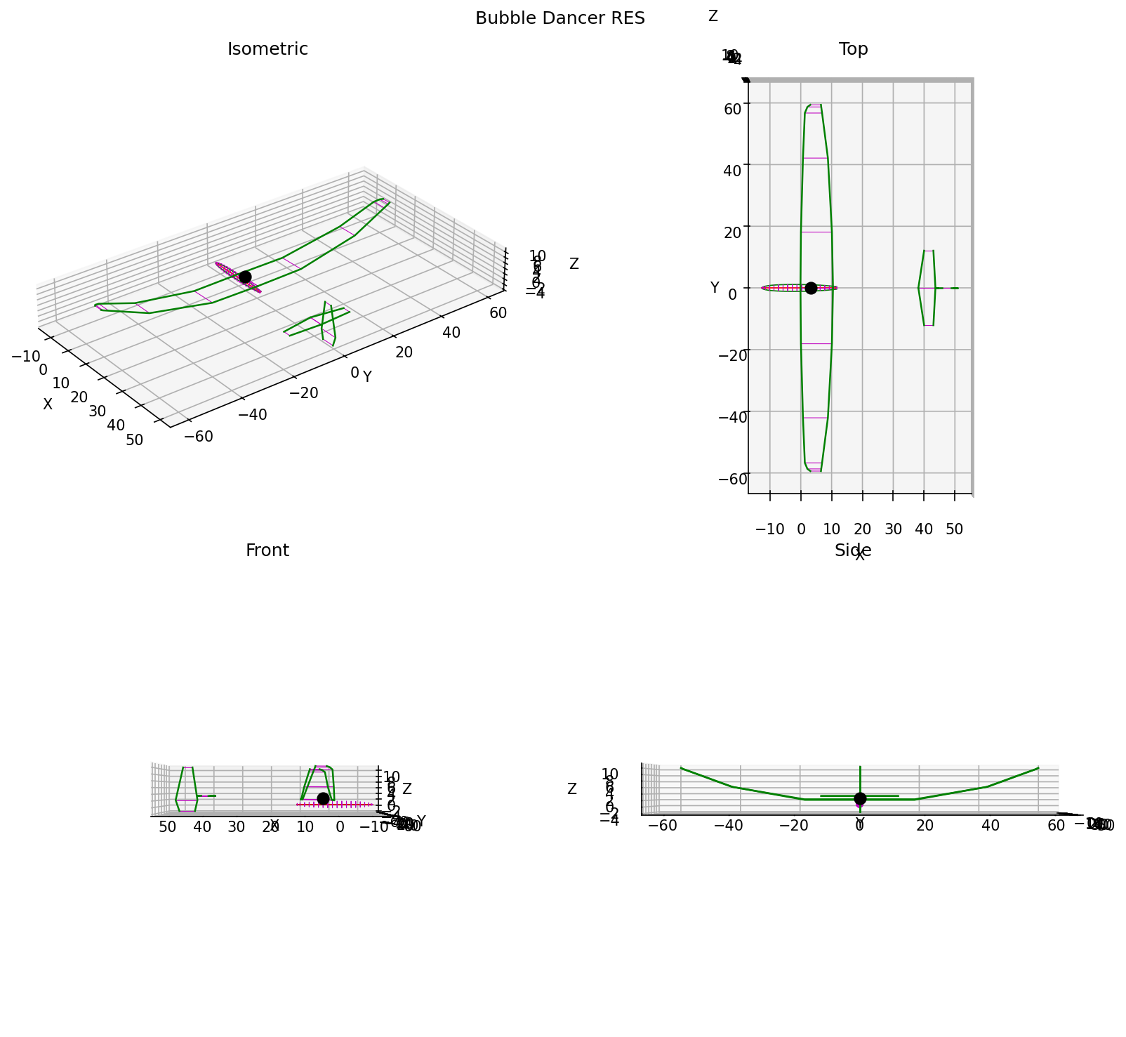
fig = avl_fileplot(geom)
fig.savefig("bd_geometry.png", dpi=150)

Bubble Dancer four-view geometry plot

Run an alpha / beta sweep#

from avl_aero_tables import avl_sweep

results = avl_sweep(
    avl_file="examples/bd.avl",
    alpha=list(range(-6, 13, 2)),   # -6 to +12 deg, 2 deg steps
    beta=[0.0],
)

print(f"{len(results)} cases computed")
for r in results[:3]:
    print(f"  Alpha={r.data['Alpha']:5.1f}  CLtot={r.data['CLtot']:.4f}")

AVL sweep complete → /your/project/out/bd/2026-05-15-143022  (10 cases)
10 cases computed
  Alpha= -6.0  CLtot=-0.1669
  Alpha= -4.0  CLtot=0.0311
  Alpha= -2.0  CLtot=0.2299

Sweep control surfaces#

results = avl_sweep(
    avl_file="examples/bd.avl",
    alpha=[-4.0, 0.0, 4.0, 8.0],
    beta=[0.0],
    ctrl_sweeps={"elevator": [-10.0, -5.0, 0.0, 5.0, 10.0]},
)
print(f"{len(results)} cases (4 alpha × 5 elevator deflections)")

Note

Surfaces in ctrl_sweeps are swept independently, not combinatorially. Two surfaces with five deflection points each produces 10 runs, not 25.

Build an aero database#

from avl_aero_tables import aero_filewrite

results = avl_sweep(
    avl_file="examples/bd.avl",
    alpha=list(range(-6, 13, 2)),
    beta=[-6.0, -3.0, 0.0, 3.0, 6.0],
    ctrl_sweeps={"elevator": [-10.0, 0.0, 10.0]},
)

aero = aero_filewrite(results)

print(aero.stab["CLtot"].data.shape)               # (10, 5) — alpha × beta
print(aero.ctrl["CLtot_d03_elevator"].data.shape)  # (10, 5, 3) — alpha × beta × defl

Important

Stability tables (aero.stab) are populated only for neutral-control runs (all deflections = 0). Include 0.0 in every ctrl_sweeps deflection list or stability tables will be empty.

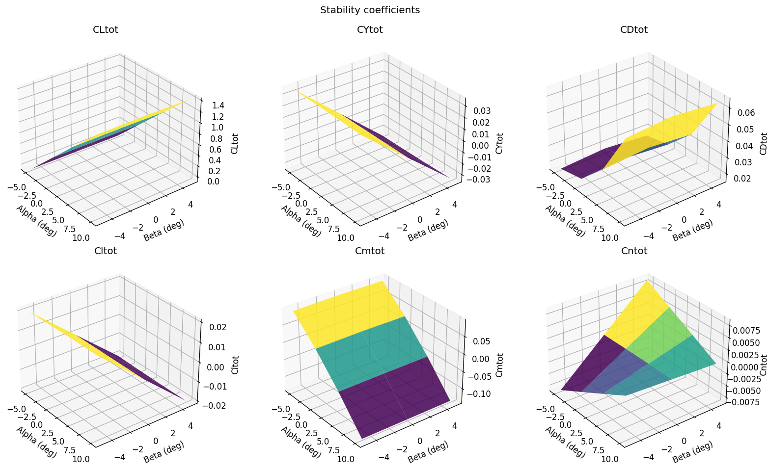
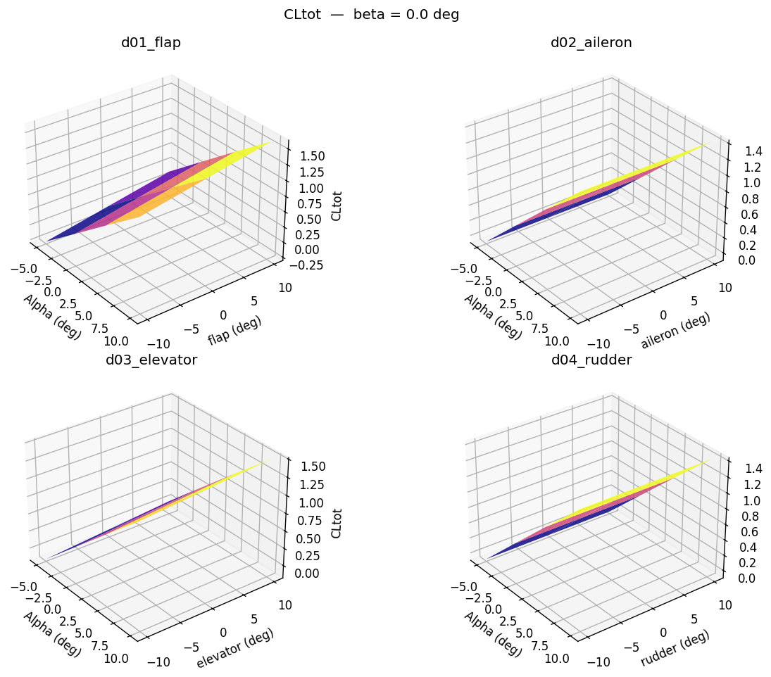
Plot the aero database#

from avl_aero_tables import aero_fileplot

figs = aero_fileplot(aero, beta_ref=0.0)
figs[0].savefig("bd_stab.png", dpi=150)        # stability coefficients
figs[1].savefig("bd_ctrl_CLtot.png", dpi=150)  # CLtot control derivatives
# figs[2..6] — CYtot, CDtot, Cltot, Cmtot, Cntot

Bubble Dancer stability derivatives

Bubble Dancer CLtot control derivatives

Geometry#

Reading a geometry file#

avl_fileread() parses an .avl file into an AvlGeometry dataclass containing a header, surfaces, and optional body definitions.

from avl_aero_tables import avl_fileread

geom = avl_fileread("examples/bd.avl")

# Header fields
geom.header.name    # geometry name string
geom.header.Sref    # reference area
geom.header.Cref    # reference chord
geom.header.Bref    # reference span

# Surfaces — keyed by surface name
geom.surface.keys()  # dict_keys(['Wing', 'Horizontal_tail', 'Vertical_tail'])

Plotting geometry#

avl_fileplot() returns a matplotlib Figure with four orthographic views.

from avl_aero_tables import avl_fileplot

fig = avl_fileplot(geom)
fig.savefig("geometry.png", dpi=150)

Running sweeps#

Alpha / beta sweep#

The primary entry point is avl_sweep(). At minimum, supply an .avl file, alpha, and beta lists.

from avl_aero_tables import avl_sweep

results = avl_sweep(
    avl_file="examples/bd.avl",
    alpha=[-4.0, 0.0, 4.0, 8.0],
    beta=[0.0],
)

Control surface sweeps#

ctrl_sweeps maps control surface names to deflection lists. Surfaces are swept independently, not combinatorially — matching the original MATLAB behaviour.

results = avl_sweep(
    avl_file="examples/bd.avl",
    alpha=[-4.0, 0.0, 4.0, 8.0],
    beta=[0.0],
    ctrl_sweeps={
        "elevator": [-10.0, -5.0, 0.0, 5.0, 10.0],
    },
)

Warning

Control surface names must match the CONTROL entries in the .avl file exactly. A KeyError is raised if a name is not found. Use geom.ctrl_names to list the available names:

geom = avl_fileread("examples/bd.avl")
geom.ctrl_names  # ['flap', 'aileron', 'elevator', 'rudder']

Output format#

The out_format parameter controls what file is written alongside the .st outputs:

Value	Behaviour
`"csv"` (default)	Writes `out_dir/results.csv`
`"json"`	Writes `out_dir/results.json`
`"df"`	Returns a DataFrame; no file written

results = avl_sweep("examples/bd.avl", alpha=[-4, 0, 4], beta=[0], out_format="json")

Output directory#

By default, each call creates a timestamped subdirectory under 📁 out/<geometry_name>/ so that previous results are never overwritten:

📁 out/
└── 📁 bd/
    └── 📁 2026-05-15-143022/
        ├── 📄 reset.run       ← AVL run-case file; all flight conditions zeroed
        ├── 📄 sweep.cmd       ← AVL command script; full stdin input fed to AVL
        ├── 📄 case_0001.st
        ├── 📄 case_0002.st
        ├── 📄 ...
        └── 📄 results.csv

reset.run is in AVL’s native .run format — the same format you would write by hand to define a run case. sweep.cmd is the complete sequence of interactive commands (one per line) that was piped to AVL’s stdin.

These two files are written before AVL is invoked, so the full inputs are always on disk alongside the outputs. To replay a run manually from a terminal:

cd examples          # must be in the directory containing bd.avl
avl < out/bd/2026-05-15-143022/sweep.cmd

To write to a fixed location instead — useful in scripts where you want to overwrite the previous result — pass out_dir explicitly. Stale .st files are removed before the new run:

results = avl_sweep("examples/bd.avl", alpha=[-4, 0, 4], beta=[0], out_dir="out/bd/latest")

Aero database#

Building lookup tables#

aero_filewrite() pivots a list[StResult] into an AeroDatabase with separate numpy arrays for stability and control derivatives.